
Using Grafana, Prometheus, and PostgreSQL
As an add-on to the project for my software engineering for AI class, I tried adding Grafana as a means of visualizing our telemetry (metrics) for our database instances, as well as our data ingestion services.
Grafana is an open source analytics and interactive visualization web application, but around the Internet it seems to be mostly used with time series data. It’s a nice all-in-one monitoring application to keep all the monitoring from different feeds and sources in one place. This is great for large production systems with many moving parts to keep track of - putting all the relevant charts, graphs, and meters in one place, rather than checking tens or hundreds of places. It’s even better when combined with alerts for when things go wrong.
In our project, we’re building a movie recommendation system for users, based on live Kafka stream of data from users watching and rating movies. In this long pipeline from stream to recommendations, anything could go wrong anywhere. It would be immensely helpful for debugging and monitoring system performance in production if we collected telemetry data about the various parts of our system, and better still collect it in one place. This motivated us to add a monitoring tool to our overall system.
Falling into the trap of beautiful graphs
Who doesn’t like beautiful graphs about metrics, especially in production ML systems? When we currently talk about observability and telemetry in systems, Grafana is often the tool that comes to be mentioned. Unfortunately I think a good number of people like me fell into this trap where we assumed that Grafana was a magic black box that would just produce amazing graphs and visualizations from our services in production. It turns out that Grafana only performs visualization - it assumes you have the telemetry data (most likely time-series data) stored nicely somewhere waiting to be visualized.
I’m not complaining, it does a great job at what it needs to do. But now I have to deal with another component, the actual telemetry collection process. This is where most roads point to using Prometheus, as our centralized all-in-one-place telemetry collection engine. Prometheus makes this entire process relatively easy and painless. For your applications and services that you wish to track, it asks only that you expose a HTTP endpoint providing the metrics you wish to collect at a single point in time. It then becomes Prometheus’s responsibility to collect data from that endpoint at a pre-specified collection interval.
That means that from the perspective of someone who already has a service or two up and running, to get metrics from those services into Grafana, you’d have to:
- Add a few lines (and I do mean a few!) of code to expose service metrics at a HTTP endpoint, and redeploy.
- Deploy Prometheus to ingest data from the endpoint we created.
- Deploy Grafana, and add the Prometheus data to the visualization.
In this post we demonstrate how to set this all up for a couple of PostgreSQL databases, as well as a custom Python service, just to show the niftiness of being able to collect multiple metrics in one place. This is especially so given that the database and the Python service are hosted in different places, and have a different stack supporting them.
Metrics from where?
Specifically, in our example, we have three things we’d like to capture data about / from.
- Metrics about our ingestion service, which continuously consumes data about users watching and rating movies from a Kafka stream, and processes the records.
- Metrics from a PostgreSQL database, where aggregated data from the ingestion service is exported to.
- Metrics from a read-only replica of the same database above, which other downstream services use e.g. for model training.
There are a number of reasons why we’d like to collect and visualize metrics for these services for our project (we’re not collecting it just for fun).
- We’d like to know how long it takes to process a batch of polled records from the Kafka stream, and if this increases or decreases over time (due to various design reasons that are beyond the scope of this article). If it takes too long, or if there’s large variance in the latency, this might suggest that our service design could be improved.
- We’d like to know on average how many queries there are from downstream services, how long queries take, and if they are too expensive to sustain. This matters since we’re deploying our PostgreSQL instances on Amazon RDS, so there’s a cost factor involved.
Data Flow
For our purposes, the telemetry data will flow in the following design.
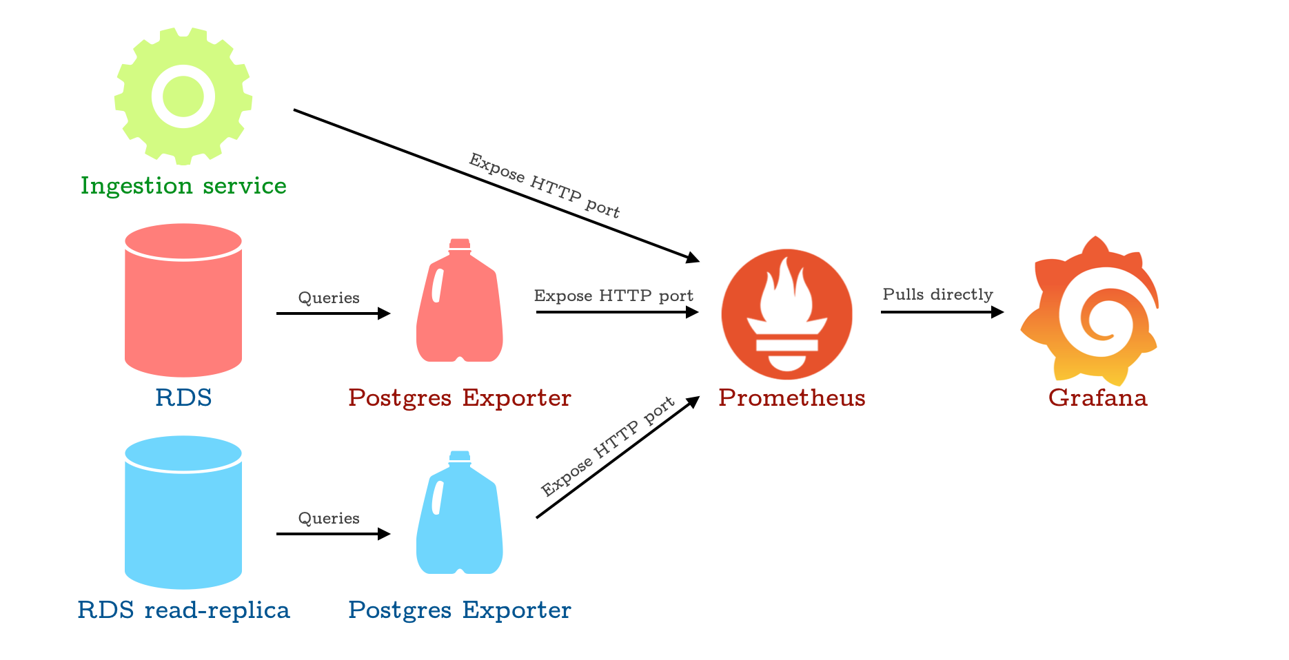
Simple infrastructure for exporting metrics eventually to Grafana. The milk jugs represent Docker containers, for the lack of a better icon. All roads lead to Grafana.
Basically, for each ’thing’ we’d like to collect data from, we expose a HTTP port. For the databases, since the databases by themselves can’t really do that, we use the Postgres Exporter service some kind soul already created to do that for us. It’s nicely packaged as a docker container, so all we have to do is specify the connection to the database and the port we intend to expose it on.
Postgres Exporter
To run the Postgres Exporter service, create an environment file with the following variables. The latter two variables are optional, it allows to specify which port and endpoint you’d like to expose.
DATA_SOURCE_NAME=postgresql://<USER>:<PASSWORD>@<HOST>:<PORT>/<DATABASE>?sslmode=disable
PG_EXPORTER_WEB_LISTEN_ADDRESS=:9188
PG_EXPORTER_WEB_TELEMETRY_PATH=/metrics
Then, docker run and you’re done!
sudo docker run -d --name rds_exporter --net=host --env-file <MY_ENV_FILE> wrouesnel/postgres_exporter
Exporting Python service data
For anything other than a database, Prometheus itself provides clients that perform the exposing of data on an endpoint. We added the Python client to our ingestion service to collect metrics about the number of new movies added, number of new users added, and the processing time for certain costly functions. We briefly describe some of them here. For example, we collect processing time metrics in the following manner:
import time
from prometheus_client import start_http_server, Summary

# Instantiate Summary object for collecting data
prom_summary_latency = Summary("processing_latency", "Latency for processing a batch of polled records")

# Start HTTP server to expose port 7070 for metrics
start_http_server(7070)

# Capturing data about our function
def our_function():
    start_time = time.time()

    # DO STUFF

    prom_summary_latency.observe(time.time() - start_time)
Setting up Prometheus
Prometheus runs in a nice Docker container. To figure out where to ingest data from, it takes in a YAML file prometheus.yml. For better management, we store prometheus.yml at /var/lib/prometheus, and map this directory to a container directory in the container so that we can change the configuration on our host.
Our prometheus.yml file looks as follows. It defines three jobs, and for each job a scraping interval and an endpoint to scrape from.
global:
  scrape_interval:     15s # By default, scrape targets every 15 seconds.

  # Attach these labels to any time series or alerts when communicating with
  # external systems (federation, remote storage, Alertmanager).
  external_labels:
    monitor: 'codelab-monitor'

# A scrape configuration containing exactly one endpoint to scrape:
# Here it's Prometheus itself.
scrape_configs:

  - job_name: 'rds'
    scrape_interval: 5s
    static_configs:
      - targets: ['<IP>:<PORT>']

  - job_name: 'rds-replica'
    scrape_interval: 5s
    static_configs:
      - targets: ['<IP>:<PORT>']

  - job_name: 'ingestion-service'
    scrape_interval: 5s
    metrics_path: '/'
    static_configs:
      - targets: ['<IP>:<PORT>']
Again, to start the Prometheus service we run the Docker container:
sudo docker run -d --name prometheus -p 9090:9090 -v /var/lib/prometheus:/etc/prometheus --expose 9090 prom/prometheus
Now, we simply visit port 9090 on the machine to see the Prometheus interface.
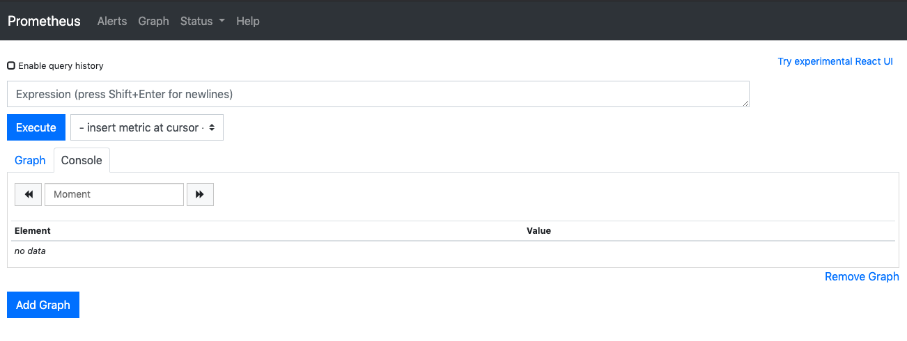
Prometheus main interface.
More importantly, navigate to the Status > Targets tab, to verify that the metrics endpoints that you are consuming are available. You should see something similar the the following.
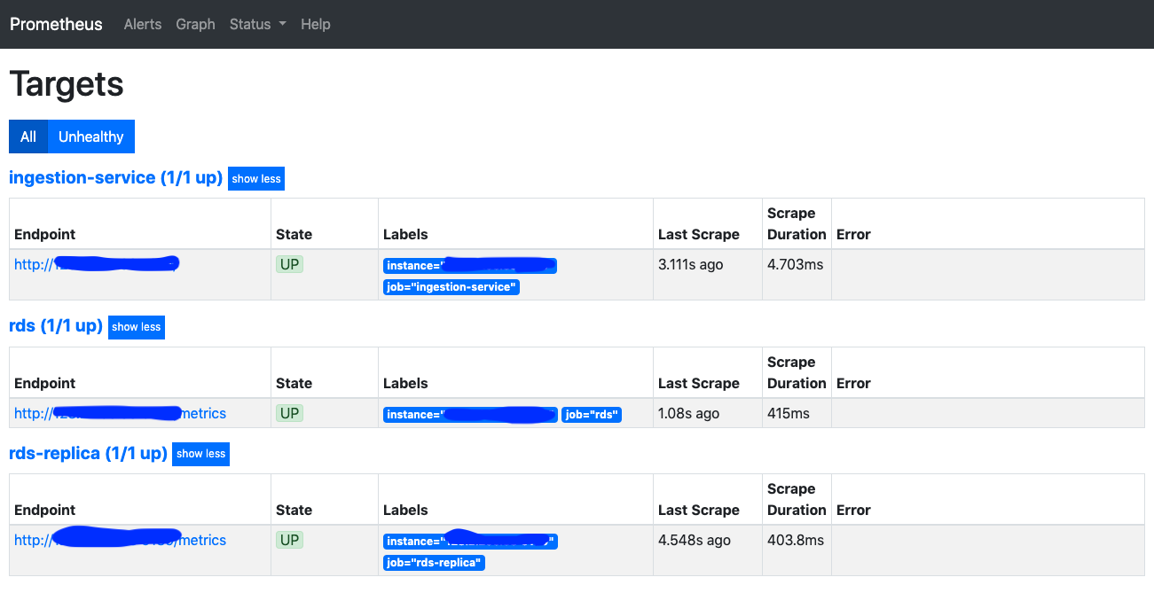
Status of metric collection targets. IP addresses obscured in a bespoke manner.
Finally Grafana
Now, we get finally get to run Grafana. To persist the settings and dashboards, we map the grafana directory of the container to a local directory.
sudo docker run -d -p 3000:3000 --name=grafana -v "/var/lib/grafana:/home/grafana/" grafana/grafana
Again, navigating to port 3000 should bring up the main Grafana interface.
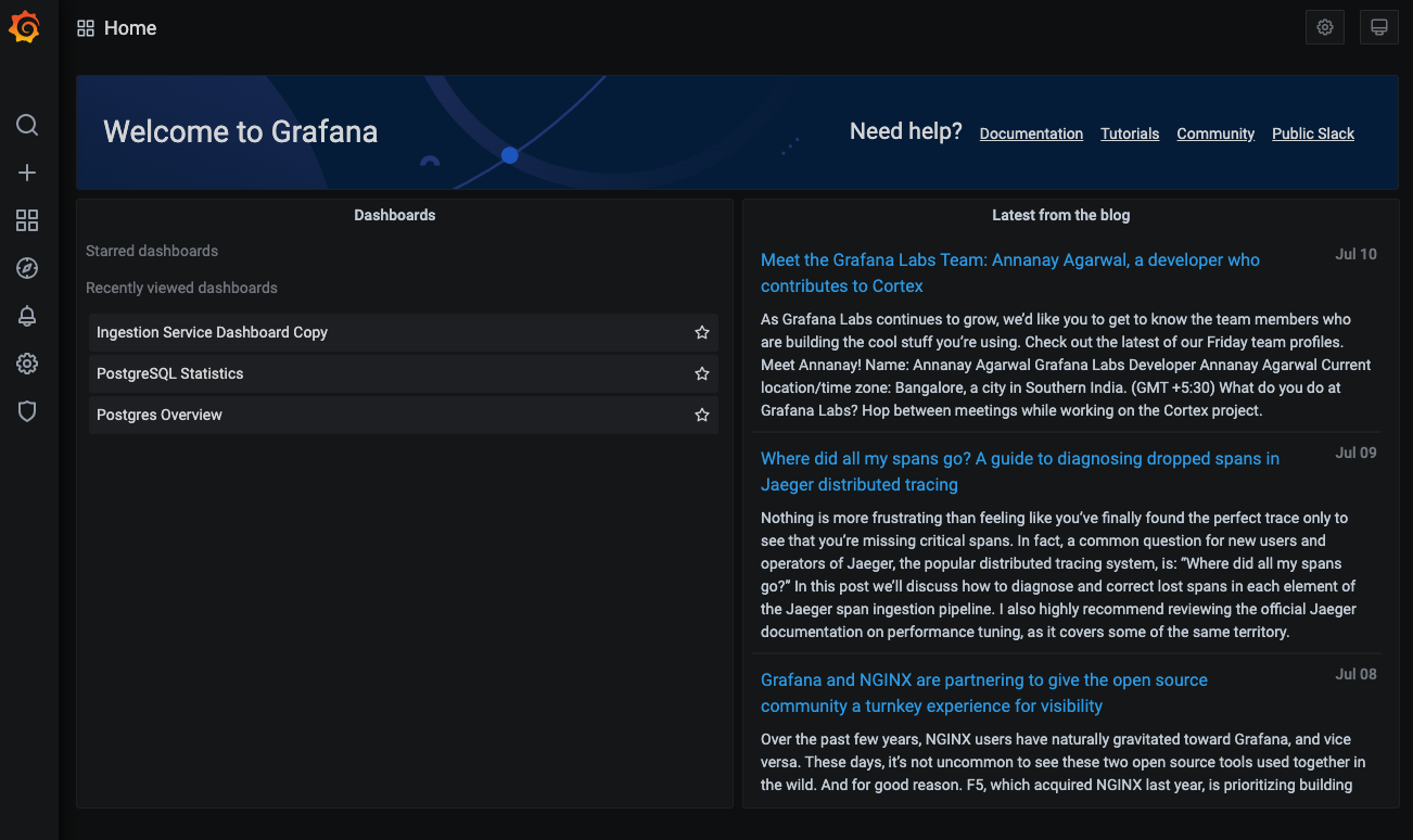
Grafana main interface with some minor advertising.
Adding Data Sources, and our first Dashboard
To visualize data from any particular source, we have to first define a Data Source in Grafana. In this case, we can navigate to the Data Source tab and add a Prometheus data source. Simply add the details for connecting to the Prometheus service (we exposed the 9090 endpoint for Prometheus earlier).
Once we’ve added the data source, we can now go ahead and create a Dashboard for our ingestion service. Dashboards here work the same way as they do on most similar software (e.g. Tableau, Metabase). We can also import dashboards designed by others, but let’s make our own first.
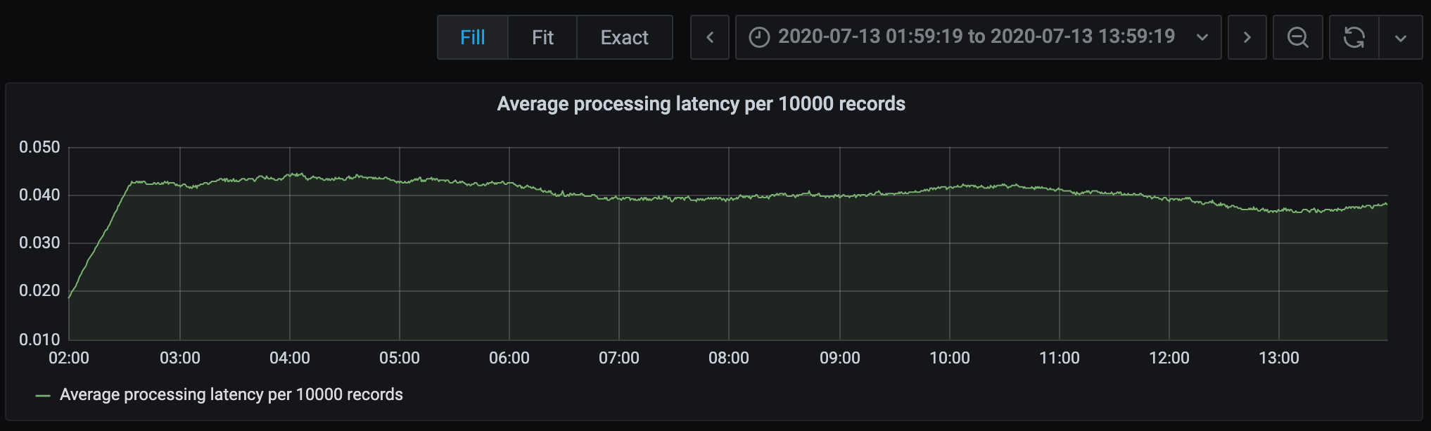
In our newly created Dashboard, click anywhere to add a new Panel. In this Panel, we select our Prometheus Data Source, and enter a Prometheus query. In this example, we want to visualize the latency of our main Kafka record processing loop. For a more representative result, we take the 1 hour running average for latency, and get the graph below.
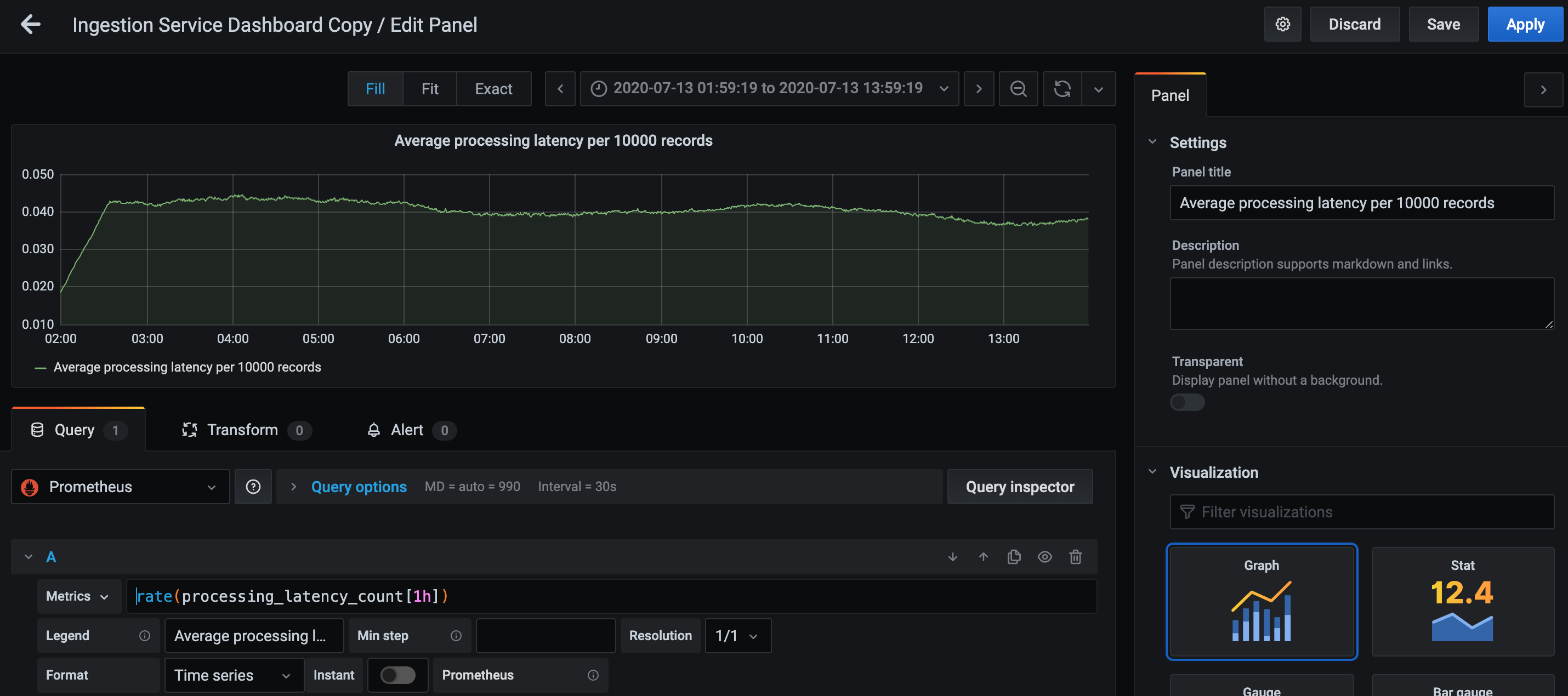
Creation of a new panel for running average latency of a target function. I left it running before sleeping, so here’s 12 hours of data.
You can actually also obtain this same graph in the Prometheus interface directly. If we enter the same query in Prometheus, we get a pretty much identical graph, barring differences and axes and timezones.
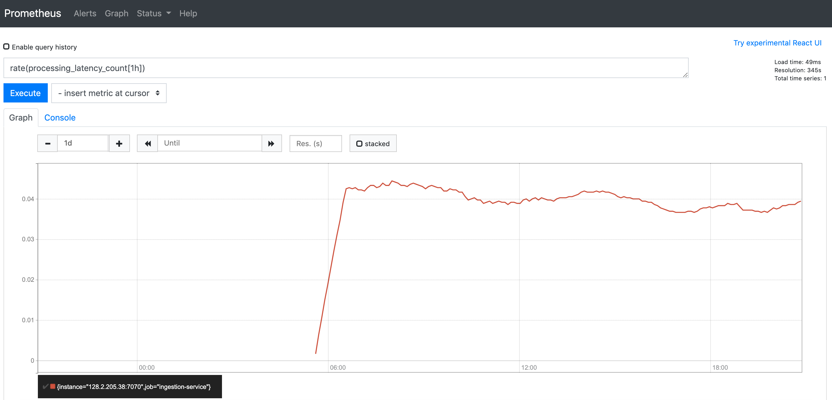
Same graph from the same query but in the Prometheus interface.
We go ahead and add two more Panels for our ingestion service dashboard, so now we can a fairly satisfying dashboard that looks like we’ve done a lot of work.
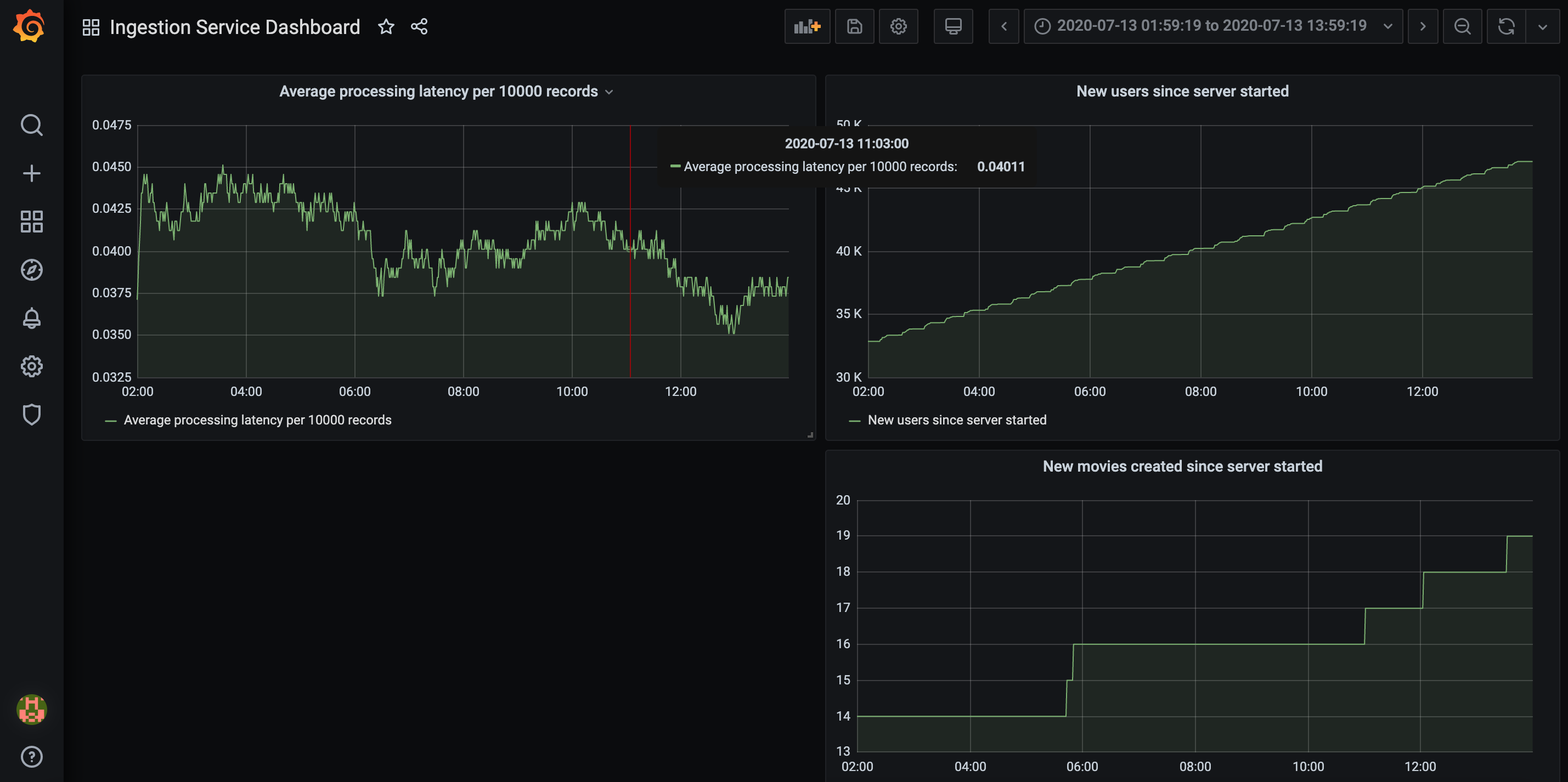
Lots of work.
I’ve added two other panels to visualize how many new movies and users we’ve added to our database from the Kafka stream since the ingestion service was started. It seems that we haven’t really added many new movies over the last 12 hours, but new users are trickling in at a relatively uniform rate.
Importing Dashboards
One cool community feature of Grafana is that Dashboards are shareable. This is very useful since more often than not, we would like to track metrics similar to what everyone else is tracking - service loads, database connections, memory consumption etc. Making a dashboard from scratch also takes a bit of effort, so why not look around to see if someone has already made one? Here we demonstrate importing a dashboard made by someone else for visualizing telemetry data from our PostgreSQL databases. We’ll use the ‘Postgres Overview’ Dashboard, which contains most of what we need. Go to Import Dashboard, and enter the ID of the Dashboard, and fill in the rest of the details.
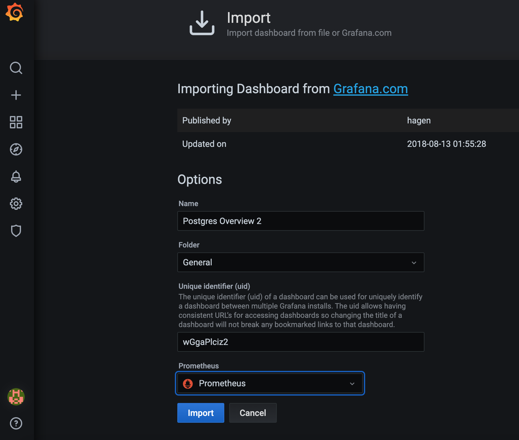
Importing a dashboard.
This should give us a relatively reasonable dashboard as follows.
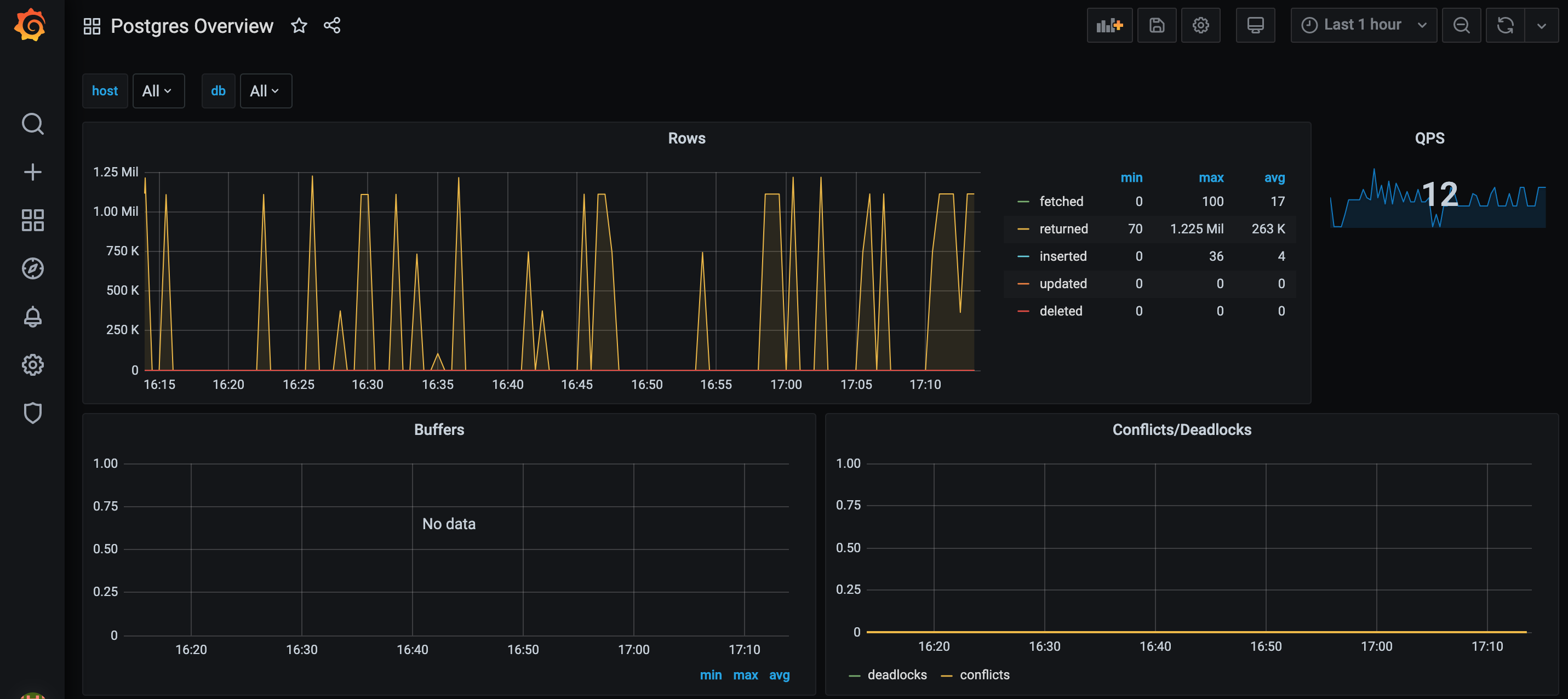
Statistics about my Postgres instance(s)! Now I just have to figure out which ones I actually need…
That’s basically it. From here its a matter of iteratively determining which metrics you need for your service, adding new ingestion endpoints to Prometheus, and producing the required visualizations in Grafana. Naturally, imported Dashboards might satisfy most but not all of your needs, so more customization likely needs to be done. For example, in the above imported Dashboard, the data is aggregated over multiple databases. If we’d like to see the data for separate databases (as in the RDS and its read-only replica), then the Prometheus queries in the Panels will need to be amended. This is still an easier process than creating it from scratch.
Comparison with Similar Tools
Grafana reminds me of Metabase (which I described in a previous post) and similar Business Intelligence (BI) tools. Apart from performance differences (Metabase got a tad slow when I added too many panels or when the SQL queries were complicated), I think a key difference between monitoring tools like Grafana and BI tools like Metabase is the source of data and the expected value-add of these systems. In monitoring tools, the data sources are often real-time telemetry streams from the various moving parts of the system. These data sources themselves are also unlikely to have direct business value, but instead reflect conditions about how the system is running in production, not unlike measuring the temperature in a machine or in a factory or in your car to determine if it is overheating or not. The purpose of such monitoring systems is also to allow developers to respond quickly to problems in the system, or to provide useful feedback to improve models and systems.
In contrast, BI tools and visualization engines often use static data e.g. from data warehouses. BI data is also often looked at after-the-fact by analysts to determine potential business insights and therefore business value, as opposed to monitoring data which looks at real-time data to diagnose potential issues within systems. As a result, BI tools often come with many useful features built-in, such as recognition of common units e.g. currency.
Nice things about Grafana
There are a few things that I do like about Grafana. The first thing is probably the large community of plugins and dashboards there are available. It is likely that for any standard software that I wish to deploy, someone has already developed a dashboard and even a data exporter for it. It is far easier fine-tuning someone else’s dashboard to fit my needs than to build one from scratch. Another thing I like about Grafana is that its interface is quite simply and easy. It was easy to setup and run, add data sources, and get started creating our visualizations. Any complexity is conveniently outsourced to other parts of the pipeline e.g. my inability to come up with good Prometheus queries is not Grafana’s problem, but it’s Prometheus’s problem.
Not so nice things about Grafana
I think the key complaint that most people have about Grafana, looking around on the interwebs, is that the data storage component has been separated entirely from the visualization process. If you recall, this is why we brought in Prometheus earlier in this example. It’s a reasonable complaint - it may not make sense to run two or three extra containers just for monitoring a simple service that may only take up one container. In fact for this example, one might argue that visualizing the queries on Prometheus was all fine and good. Granted, you couldn’t have many graphs on one page and it didn’t look as fancy, but it may have well been sufficient for the job. In the end, I think it comes down to a matter of scale. Personally I quite like the separation between visualization and data collection, and I think I’ll keep it that way.